Bayesian statistical methods can make predictive data analysis more accurate. In this article, we evaluate possible solutions to the challenge of refining and increasing the value of high-volume data streams.

When dealing with an overwhelming amount of data, it is often beneficial to process the data locally as it is collected, at the device level. Take for example the common case of IoT devices continuously providing sensor data: current location and temperature, accelerometer readings, light and humidity levels. All this information is likely to be sent at high frequency and be very “noisy.” Data like this could be consumed by user-facing applications or used to train machine learning/AI algorithms to provide additional insights, but those uses will be much more effective if the data is cleaned up and enriched before processing.

What kind of “enrichment” is useful? We might want to know if the observation is anomalous, i.e., outside a quantifiable threshold. We might want to use de-noised data. We might want to use a short-term prediction for a time series, or we might want a method to interpolate missing points. Bayesian methods provide tools that can answer these questions in many scenarios. We will look at some of these available methods, but first, we’ll define some of our terms.

Bayesian methods provide tools that can answer these questions in many scenarios.

Real time refers to methods that can provide a result within a fixed, bound computational time and that are compatible with a human perception of real time, e.g., in the sub-second scale. Real-time estimation is also a necessity when dealing with inference in the context of potentially mission-critical systems, such as self-driving cars, drones, or any other system that requires an “always on” state, usually with a high-frequency input of data.

Online means an inference method that takes one observation, or at least a fixed window of observations, into account. That is, we want our inference method to be O(1) relative to the number of observations, without growing in computational cost as time goes by (e.g., as a result of having to process historical data). As a practical example of an online method, we can consider filtering location and position data from a car’s GPS. We wouldn’t expect the computational cost to grow unbounded as we drove for longer!

Having a strong statistical underlying foundation is also essential if we want to be able to make critical decisions based on error margins or confidence of our estimations. For instance, if a sensor is missing a few observations, we can carry forward the state and quantify the prediction’s confidence interval. Also, we might want to classify an observation as an outlier if it falls outside a quantifiable threshold. These tasks are simple to perform if we choose the appropriate model for our data.

Particle filters as a possible solution

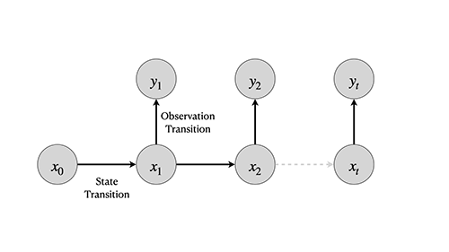
A standard way of performing estimation on time series and guaranteeing the online property is to use state-space models (SSMs). In state-space models, we assume that an underlying hidden state evolves in time and that at each time point we measure an observation. SSMs possess a Markovian nature; that is, at each time point, the current state only depends on the previous state and model’s parameters, and observations rely on the current state and model’s parameters.

For a specific class of models where we assume linearity, i.e., an underlying Gaussian posterior for both state and observation transitions, some classic and exceptionally well-researched solutions are available, e.g., the venerable Kalman Filter (KF) introduced by Kalman et al. in 1960.The KF provides the optimal solution for this model family. But even in the case where we don’t have a linear system, there are other variants of the KF, such as the Extended Kalman Filter (EKF). Proposed by both Jazwinki (1966) and Maybeck (1979), the EKF can be used by approximating the non-linear transitions with a first-order Taylor Series. However, different approaches are available that neither assume state model linearity or unimodal posteriors, nor rely on local linearization.

One such solution is called Particle Filters (PF), also commonly known as Sequential Monte Carlo (SMC), a well-established method of Bayesian inference based on importance sampling. These methods have been well researched since the latter part of the twentieth century. They have been increasingly adopted in a multitude of scenarios in recent years, made possible with the advent of increased computational power.

In a nutshell, PFs estimate a sequence of underlying states, as defined by our SSM. 

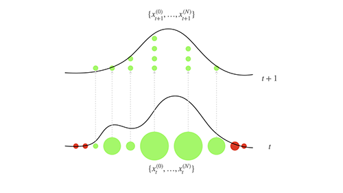
In a nutshell, PFs estimate a sequence of underlying states, as defined by our SSM. This is done by propagating a certain number of particles according to a state transition. Numerous algorithms are available, but in a standard PF (e.g., Sequential Importance Resampling [SIR]), we resample particles according to their weights, provided by the observation’s likelihood, and the resulting particles are propagated further. 

The underlying concept is to try to explore the state-space as efficiently as possible, thrusting particles forward and creating an approximation of the state’s posterior. Although theoretically the PF estimation error converges to zero as the number of particles increases to infinity, in the real world we are dealing with a finite (and sometimes extremely constrained) number of particles. The strategy therefore is to select the particles with a higher likelihood, according to our observation model, and duplicate them. With a finite number of particles and without resampling, most of the weights would eventually be zero. 

So how is the state estimation determined from this set of particles? Depending on the implementation used, we can choose a weighted mean of the particles or a single particle with the highest weight.

The problem of particle impoverishment

Although PFs provide the framework for online state estimation in SSMs, we need to define our transition and observation models. PFs coupled with a flexible, elegant way of defining our underlying transition and observation model, such as the Dynamic Generalised Linear Models (DGLMs), provide a compelling solution.

DGLMs allow us to model complex time-series behaviours by composing simple patterns into more complex ones. We have, for instance, components for linear and polynomial trends, as well as cyclic trends represented by Fourier components. We assume a linear state transition, but can now associate it with a linear or nonlinear observation model. This gives us the ability to model a wide variety of data—e.g., both continuous and discrete data with complex cyclic patterns.

Special consideration must be made, however, when using PFs for low-powered hardware, such as that typically found in IoT devices. An obvious issue is that computational requirements grow linearly with the number of particles and also grow with the state-space dimensions. A tradeoff must be made between the computational cost and the estimation error, as well as the model’s complexity. As an example, is it necessary to incorporate a yearly seasonal component in a temperature data stream model, if the time-series granularity is the order of a measurement every second?

In any case, the act of resampling the particles introduces a problem usually termed particle impoverishment. If we think of selecting a portion of particles with higher likelihood and discarding the remaining ones, we are throwing away information. After a few iterations, all the particles will have a single ancestor. This is problematic since we now are not exploring the state-space as efficiently as possible.

Clearly, these two problems—computational costs and reducing particle impoverishment (especially important for long-running time-series data as we might find in IoT devices)— constitute two of the biggest challenges when implementing local stream processing in low-powered devices. We will look at some of the potential solutions.

With modern high-end hardware, we could simply use a massive number of particles. This might not necessarily introduce a computational cost problem, since PFs are notoriously, embarrassingly parallel in the state propagation phase (i.e., each particle can be propagated independently, in parallel), and this property could be further exploited with modern hardware architectures, such as high numbers of CPUs, as well as GPUs.

With modern high-end hardware, we could simply use a massive number of particles. 

This is, however, problematic in low-powered devices. Additionally, increasing the number of particles will only delay the problem; we are just postponing the inevitable particle impoverishment, and the computational costs will be prohibitive. Solutions will have to rely on theoretical advancements, rather than just brute force calculations.

Another consideration is that, so far, we have assumed that for “standard” PFs, we are only interested in estimating the state. But that implies that we are assuming that we know the state and observation’s transition model parameters. This is often not the case.

The estimation becomes even more complex when we are trying to estimate the model’s states and parameters simultaneously. And this may very likely be the real-world scenario we are dealing with. 

How SMC2 could help

Over the years, a considerable amount of research has been made into the state and parameter estimation. A promising solution is to use methods such as SMC², as introduced by Chopin et al. (2013). SMC² provides the ability to estimate both states and parameters. However, this requires the ability to calculate the observation’s incremental likelihood at each time point, which, for most models, won’t be possible in an analytical way. Crucially, Standard PFs (e.g., SIR) provide an unbiased estimator of the marginal likelihood and can be used as “parameter” particles. This nested PF-within-a-PF approach is alluded to in the name SMC-squared. 

Since, as mentioned earlier, SIR filters rely on the assumption that the parameters are known, we condition each of these Parameter PFs on a particular parameter value. A degeneracy threshold is established, and if that threshold is crossed, then the parameter particles are resampled. The resampled particles can then be propagated using a Particle Markov chain Monte Carlo method (PMCMC) step, such as Particle Marginal Metropolis-Hastings (PMMH) or Particle Gibbs. This step is essential to the algorithm because it permits performing a particle “rejuvenation” by using a PMCMC kernel, which can greatly help to mitigate the problems of particle impoverishment. However, because this rejuvenation step uses previous data, it ceases being an online method (although it is still a sequential method), requiring the storage of past stream data points.

However, it is possible to keep the computational cost bound per iteration, by targeting an approximate distribution  and evaluating the PMCMC for a fixed window of recent observations. Ad-hoc implementations, such as O-SMC², allow use of the flexible and model-agnostic advantages of SMC² while keeping the sequential andonline requirements for streaming data.

Another potential solution to be considered is the state augmentation family of PFs. One example is Particle Learning (PL), as presented by Carvalho et al. (2010). This approach uses an essential vector, a vector of sufficient statistics that summarises the model state used for the state and parameter propagation itself. If each particle has an associated set of sufficient statistics, these can be individually updated, at each time-step, in a deterministic way. This has the obvious advantage of providing a low computational cost due to the low dimensionality of the sufficient statistic vector. Additionally, provided sufficient statistics are available, this marginalisation of the state and parameters can help fight particle degeneracy. In benchmarks, PL methods provided a reasonable approximation to the true state (estimated offline, using a gold standard such as PMMH). 

Methods such as O-SMC² provide attractive features, such as the ability to apply to a huge variety of models, lower estimation error, particle rejuvenation, and being implementation agnostic. However, the computational cost might be too high for low-powered devices dealing with high-frequency data, in the magnitude of at least a few seconds for each time point on modest hardware. For streaming data with lower frequency (e.g., data points every minute), it might be a compelling option. Sufficient-statistics based methods, such as PL, provide a reasonable real-time estimate, and in theory should delay particle impoverishment issues, at the cost of a few hundred milliseconds per iteration. This is especially the case when our models are simple (i.e., few state components), for instance, for temperature estimation or motion estimation.

In summary, although theoretical research is extremely active in the field of real-time, online state and parameter estimation for streaming data, if the goal is to provide the best possible estimates, PFs are still not a match for offline methods such as the Markov chain Monte Carlo method. However, if the goal is to have a reasonable estimation sufficient for IoT data processing, PFs offer a compelling, flexible, and robust solution, with methods that provide strong candidates for further research in this field.

References

Andrieu, C., Doucet, A. and Holenstein, R. (2010). “Particle Markov chain Monte Carlo methods.” Journal of the Royal Statistical Society. Series B: Statistical Methodology 72 (3), 269–342. 

Carvalho, C.M., Johannes, M.S., Lopes, H.F. and Polson, N.G. (2010). “Particle learning and smoothing.” Statistical Science 25 (1), 88–106.

Chopin, N., Jacob, P. E. and Papaspiliopoulos, O. (2013). “SMC²: An efficient algorithm for sequential analysis of state-space models.” Journal of the Royal Statistical Society. Series B: Statistical Methodology 75 (3), 397–426. 

Jazwinski, A. (1966). “Filtering for nonlinear dynamical systems.” IEEE Transactions on Automatic Control 11 (4), 765–66.

Kalman, R. (1960). “A new approach to linear filtering and prediction problems.” Journal of Basic Engineering 82, 35–45

Maybeck, P. S. (1979). Stochastic models, estimation, and control, vol. 1.

Vieira, R. (2018). “Bayesian online state and parameter estimation for streaming data.” PhD diss., Newcastle University. http://theses.ncl.ac.uk/jspui/handle/10443/4344

Vieira, R., and Wilkinson, D. (2016). “Online state and parameter estimation in dynamic generalised linear models.” arXiv preprint arXiv:1608.08666.