


























Researchers are proving that small open source models, using a well-established algorithm, can compete successfully with proprietary frontier models.
Large language models continue to improve through larger architectures and more training data, but recent evidence suggests diminishing returns from scaling model size alone. A complementary approach—inference-time scaling (ITS)—allocates more computation during inference to improve performance without increasing model parameters. Existing ITS methods such as beam search and diverse verifier tree search (DVTS) treat inference as a search problem guided by a process reward model (PRM), a separate neural network that scores each intermediate reasoning step. But these methods trust the PRM deterministically, pruning any path that scores poorly—even if the score is wrong. In our NeurIPS 2025 paper “Rollout roulette: a probabilistic inference approach to inference-time scaling of LLMs using particle-based Monte Carlo methods,” we show that a three-decade-old algorithm from signal processing—particle filtering (one of the Sequential Monte Carlo methods)—offers a principled alternative that treats reward scores as uncertain evidence rather than ground truth.
The filtering problem
Imagine a cruise ship navigating through dense fog. The ship has a GPS sensor, but it is noisy—each reading scatters around the true position by some unpredictable amount. If you plot the raw GPS readings, you get a jagged, wandering path that only loosely resembles the ship’s actual trajectory.
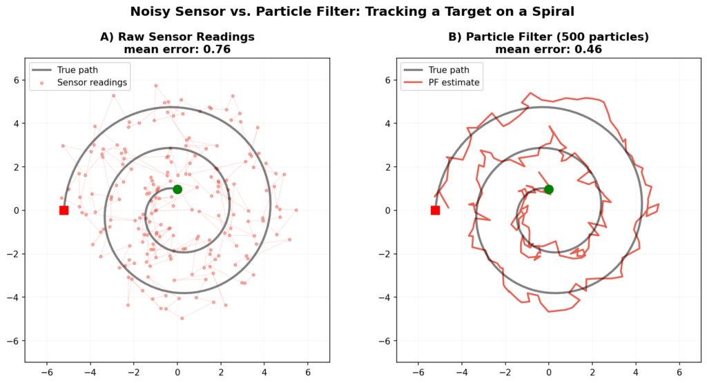
Here is the surprising part: particle filtering can track the ship more accurately than the GPS sensor itself, by learning from the same sensor data. In an example simulation we ran—a target moving along a 2D spiral over 200 time steps with Gaussian sensor noise (standard deviation 0.6)—a particle filter with 500 particles and a velocity model achieved a mean tracking error of 0.46, compared to 0.76 for the raw sensor (see Figure 1). That is a 39% improvement, using only the same noisy readings as input. This ability—producing better estimates than the sensor it relies on—is why particle filtering appears in robot localization, submarine navigation, and aircraft tracking.
How particle filtering works
You want the true position of the ship, but you cannot observe it directly. You have two imperfect tools: a motion model that generates candidate positions for where the ship might be next, and a GPS sensor that scores each candidate. The algorithm repeats three steps at each time step:
- Propagate: push each particle (candidate position) forward using the motion model.
- Score: weight each particle based on how well it matches the latest sensor reading.
- Resample: stochastically select particles for the next round. High-scoring particles are more likely to survive, but low-scoring ones are not guaranteed to die.
Why does this beat the sensor? Because the sensor is noisy, and particle filtering treats its readings as uncertain evidence rather than ground truth. If you deterministically kept only the top-K particles by sensor score at each step, the population would collapse into near-identical clones within a few steps—locked onto wherever the GPS noise happened to point. One bad reading, and the entire population drifts off course with no way to recover.
Stochastic resampling prevents this. High-scored particles are favored but not guaranteed to survive; low-scored particles can persist. A particle that looks mediocre now might be the only one near the true position three steps later. The population stays diverse enough to recover from scoring errors, rather than committing prematurely to whatever the noisy sensor happens to favor at any given step.
Particle filtering for LLM reasoning
Now replace the cruise ship with a hard math problem. You want the correct solution, but you cannot generate it directly—if you could, the problem would already be solved. You have two imperfect tools, structurally identical to the filtering setup above.
The LLM serves as the transition model: given a partial solution, it generates the next candidate reasoning step. A process reward model (PRM) serves as the emission model: it scores each intermediate step for correctness, like a grader reading the LLM’s work line by line. But the PRM is noisy. In Figure 2, we show a real example where the PRM assigns a score of 0.9453 to the first step of a wrong answer and only 0.5156 to the first step of the correct answer. Any method that trusts these scores deterministically would immediately prune the correct solution.
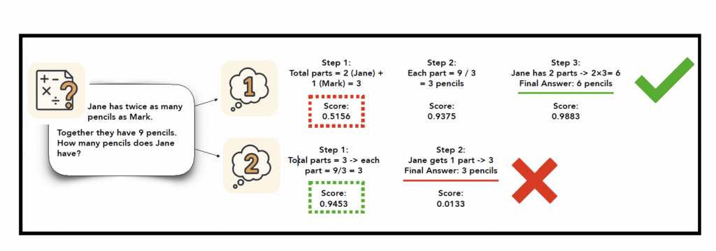
This is exactly what beam search does. It keeps the top-K highest-scored partial solutions at each step and discards the rest. One bad score early on, and the correct path is gone permanently. Best-of-N takes a different but equally brittle approach: generate N complete solutions independently, then pick whichever the PRM scores highest overall. It treats the reward model as ground truth and has no memory across reasoning steps—each solution is produced in isolation.
Our method formulates ITS as approximate posterior inference over a state-space model (Figure 3). Each particle is one partial reasoning path. At each reasoning step, we propagate (extend each path with the LLM), score (evaluate with the PRM), and resample (select paths via softmax-weighted stochastic sampling). The softmax resampling is the critical difference from beam search: low-scored paths can survive, and high-scored paths are favored but not guaranteed. This preserves population diversity and allows recovery from noisy early scores.
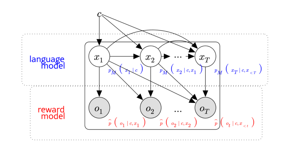
The parallel to classical filtering holds precisely. Just as the particle filter tracks a ship’s position more accurately than the GPS sensor it relies on, our method finds correct solutions more reliably than the noisy PRM it uses for scoring. With prefix caching, the runtime is comparable to generating N full completions independently.
Results
We performed our experiment on the MATH500 dataset, a set of 500 complex math problems used in the AI community to evaluate the mathematical reasoning capabilities of language models. Small open source models combined with particle filtering compete directly with frontier proprietary models. Figure 4 shows the outcomes. Qwen2.5-Math-1.5B—a model small enough to run on modest hardware—paired with particle filtering achieves 84.6% on MATH500 with a budget of 32 generations, surpassing GPT-4o (76.2%) with a budget of only 4. At the 7B scale, Qwen2.5-Math-7B with particle filtering reaches 87.7% on MATH500, matching o1-preview (87.0%) at budget 32. On AIME 2024, a notoriously difficult competition benchmark, it achieves 10/30 compared to 7/30 for beam search.
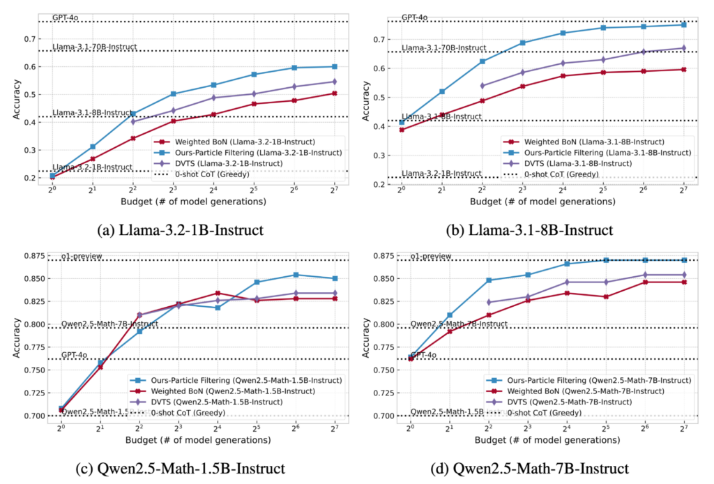
Particle filtering also scales more efficiently than alternatives. DVTS, the next best competitor, requires a budget of 32 to match what particle filtering achieves at budget 8—a 4-16x efficiency advantage. On non-math-specialized models, the gains are equally clear: Qwen2.5-1.5B (a general-purpose model) reaches 79.3% on MATH500 with particle filtering versus 76.2% for beam search and 76.6% for DVTS. The method also generalizes beyond mathematics: on FinanceBench, particle filtering achieves 70.33% versus 67.33% for beam search, and on NumGLUE Chemistry, 84.22% versus 80.47%.
What this means
For engineers running models in production, the takeaway is practical: a smaller model with principled inference-time scaling can match or exceed the performance of a much larger one at a fraction of the serving cost. And the algorithm enabling it is not new, but a well-understood technique from signal processing, applied to a problem where it turns out to fit remarkably well. Sometimes the best ideas in AI are the ones we already had.